Speeding Up Sum-Check Proving

Speeding Up Sum-Check Proving (Bagad et al.)

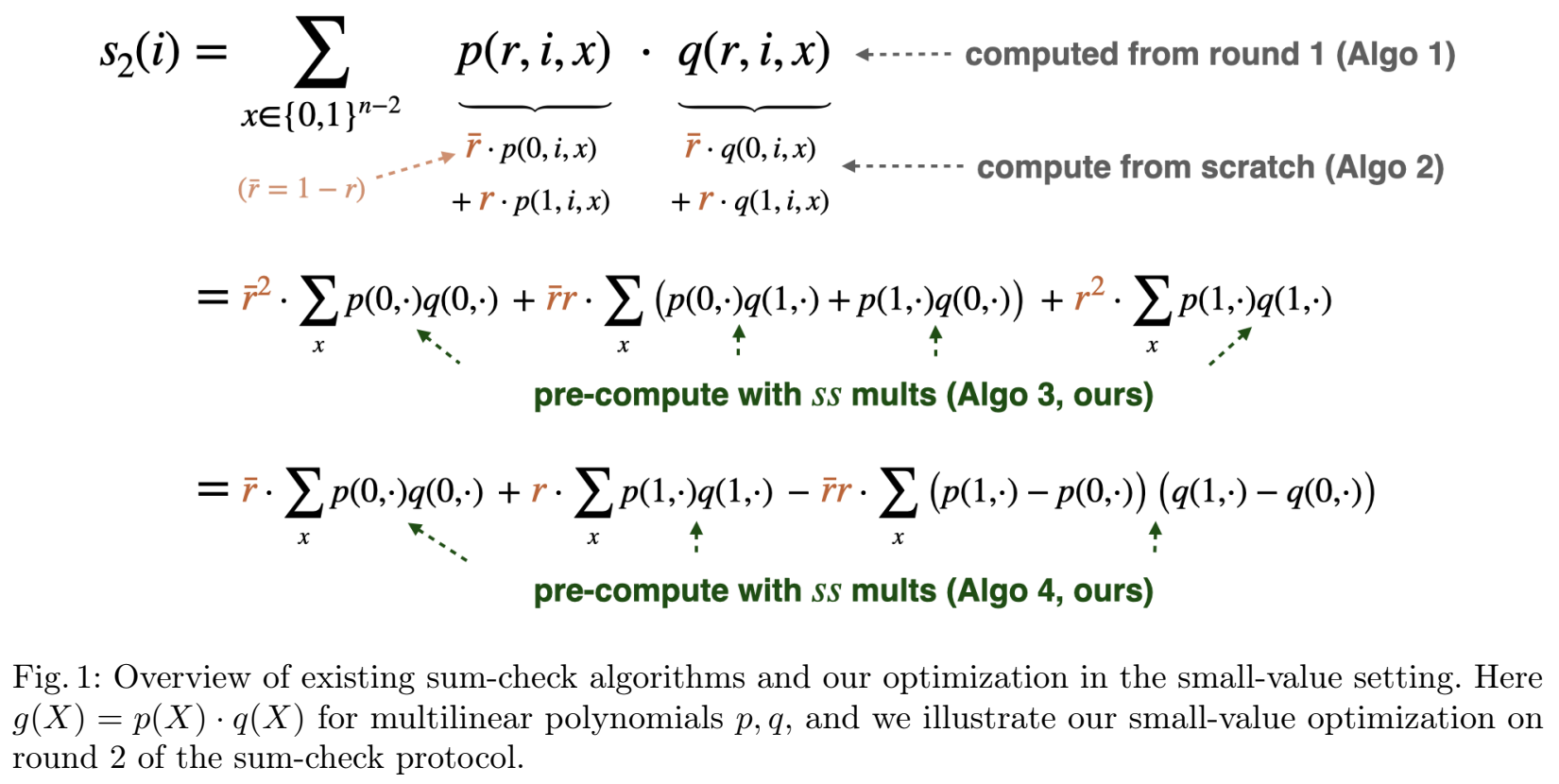
TLDR: Recaps existing proving algorithms, introduces new algorithm to (1) trade off multiplications between large field elements (expensive) for multiplications between small field elements cheap, and (2) optimize for the common case where $g$ has $\widetilde{eq}(r,X)$ as one of its factors, as common in Spartan and Jolt.

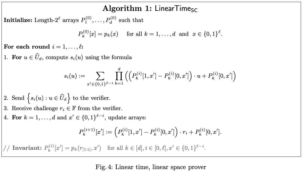
Algorithm 1: Linear time & space prover

Proves ${\sum }_{x\in \{0,1{\}}^l}g(x)=C_0$ for an $l$-variate polynomial $g$ which is a product of $d$ multilinear polynomials:

$$g(X)=p_1(X)\cdot ...\cdot p_d(X)$$

The degree-$d$ univariate polynomials sent to the verifier as part of the Multivariate Sum-Check Protocol are represented by their evaluations on a fixed set of $\widehat{U_d}$.

Their definition of $\widehat{U_d}$

They define $U_d:=(\infty ,0,1,2,...,d-1)$ and $\widehat{U_d}:=U_d\setminus \{1\}$. For a polynomial $s$, $s(\infty )$ is defined as the highest degree coefficient of $s(X)$. Lemma 2.2 shows how to do Lagrange interpolation in this setting. I’m not sure what’s the advantage over using e.g. $U_d:=(0,1,2,...,d)$.

Notes:

• The algorithm starts out by storing the polynomials $p_k(X)$ (for $1\le k\le d$) in evaluation form in arrays $P_k^{(0)}$ of size $2^l$ each.
• Step 4 computes $P_k^{(i+1)}$ (of size $2^{l-i-1}$) from $P_k^{(i)}$ (of size $2^{l-i}$) to maintain the stated invariant, binding one variable to the verifier challenge. The update uses the fact that for any multilinear polynomial $p$, we have $p(r,x)=(1-r)\cdot p(0,x)+r\cdot p(1,x)$. This allows us to bind the variable to any value.
• Step 1 can be broken down as follows:
  • The prover message is a univariate polynomial $s_i(X)$, whose representation is computed by evaluating $s_i(u)$ for all $u\in \widehat{U_d}$
  • $s_i(u)$ is computed as ${\sum }_{x^{\prime }\in \{0,1{\}}^{l-i}}g(r_{[1:i]},u,x^{\prime })$
  • $g(r_{[1:i]},u,x^{\prime })$ is computed as ${\prod }_{k=1}^d{p}_k(r_{[1:i]},u,x^{\prime })$
  • $p_k(r_{[1:i]},u,x^{\prime })$ is computed from $p_k(r_{[1:i]},0,x^{\prime })$ and $p_k(r_{[1:i]},1,x^{\prime })$ (both stored in $P_k^{(i)}$) using the same fact used in in step 4

Notes on performance:

• In each round, the main memory usage is $d$ size-$2^{l-i}$ field elements. Note that in practice, these field elements are usually small in the first round and large after (because they depend on a random challenge).
• The number of multiplications halves in each round, but from round 2, the multiplications are between large field elements.

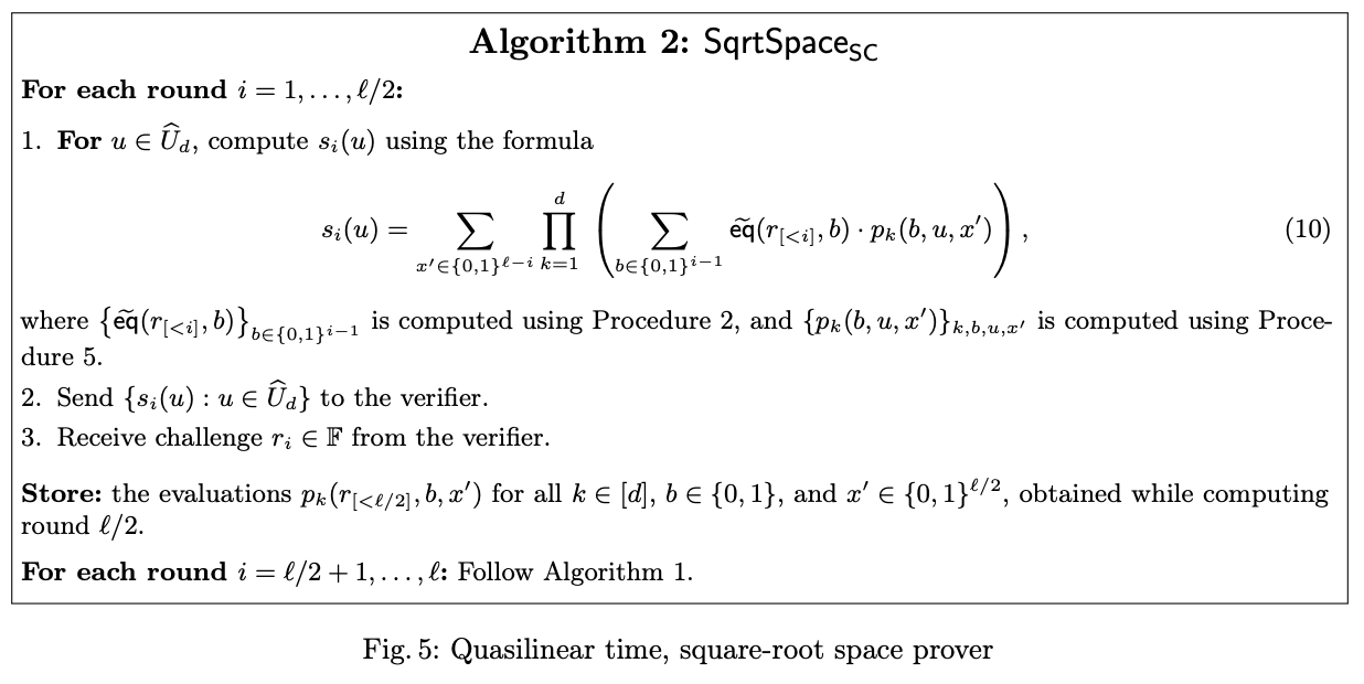
Algorithm 2: Quasilinear time & square-root space

The core idea of this algorithm is that the terms $p_k(r_{[1:i]},u,x^{\prime })$ (where $r_{[1:i]}\in {\mathbb{F}}^{i-1}$, $u\in \widehat{U_d}$, $x^{\prime }\in \{0,1{\}}^{l-i}$) can also be computed directly from the evaluation form of $p_k$: Notes:

• The evaluation form of polynomials $p_k$ can be accessed sequentially. This enables a streaming prover: Witness generation is re-run for each of the first $l/2$ sum-check rounds; the prover never has to store the entire witness.
• The $\widetilde{eq}(\cdot ,\cdot )$ terms can be computed in linear time. The time and space needed is $2^{i-1}$, i.e., at round $l/2$, this array will have $2^{l/2-1}=\sqrt{2^l/2}$ elements.
• After $l/2$ rounds, the prover switches to Algorithm 1. At this point, the arrays $P_k^{(l+1)}$ contain $2^{l/2}=\sqrt{2^l}$ elements.

Notes on performance:

• Memory usage is $O(\sqrt{2^l})$
• The inner product is between a large field element (the $\widetilde{eq}(r_{[<i]},b)$ term) and a small field element (the $p_k(b,u,x^{\prime })$)
• The outer product is between large field elements (after round 1)